<?xml version="1.0" encoding="utf-8"?><feed xmlns="http://www.w3.org/2005/Atom" ><generator uri="https://jekyllrb.com/" version="3.10.0">Jekyll</generator><link href="https://fullfix.github.io/feed.xml" rel="self" type="application/atom+xml" /><link href="https://fullfix.github.io/" rel="alternate" type="text/html" /><updated>2026-04-21T20:29:29+00:00</updated><id>https://fullfix.github.io/feed.xml</id><title type="html">Nikita Breskanu Research Blog</title><subtitle>Research notes on deep learning optimization &amp; compression.</subtitle><entry><title type="html">Fisher-based Optimizers in Deep Learning</title><link href="https://fullfix.github.io/notes/2026/04/21/fisher-optimizers.html" rel="alternate" type="text/html" title="Fisher-based Optimizers in Deep Learning" /><published>2026-04-21T00:00:00+00:00</published><updated>2026-04-21T00:00:00+00:00</updated><id>https://fullfix.github.io/notes/2026/04/21/fisher-optimizers</id><content type="html" xml:base="https://fullfix.github.io/notes/2026/04/21/fisher-optimizers.html"><![CDATA[<p>This post summarizes the natural-gradient view of deep learning optimization and reviews practical Fisher-based approximations for linear layers in chronological order. The central question is how methods such as KFAC, EKFAC, Shampoo and SOAP make structured preconditioning cheap enough to use in neural networks.</p>

<!--more-->

<h2 id="introduction">Introduction</h2>

<p>Optimization is one of the most important aspects of deep learning. It is non-convex, highly stochastic, and strongly anisotropic, which creates a gap between clean optimization theory and the practice of training large neural networks. Standard first-order methods such as stochastic gradient descent are often insufficient for modern large-scale training [<a href="#amari1993backpropagation">Amari 1993</a>].</p>

<p>The default optimizer in many deep learning pipelines is Adam or AdamW [<a href="#kingma2014adam">Kingma and Ba 2014</a>]. Adam is powerful and robust, but it is mostly structure-agnostic: it treats parameters coordinate-wise and ignores the fact that most weights in modern networks live inside linear layers. Fisher-based optimizers try to use this matrix structure to approximate natural-gradient updates without forming the full Fisher matrix.</p>

<p>We consider a discriminative task of the form</p>

\[\mathcal{L}(w)
=
\mathbb{E}_{(x,y)\sim \mathbb{D}}\, l(f_w(x), y)
\to
\min_w,\]

<p>where $w \in \mathbb{R}^D$ are model parameters and $f_w(x)$ are logits. For a negative log-likelihood loss,</p>

\[l(f_w(x), y)
=
-\log p(y \mid f_w(x))
=:
-\log p_w(y\mid x),\]

<p>the optimization problem can be viewed as maximum likelihood estimation.</p>

<h2 id="natural-gradient">Natural Gradient</h2>

<p>The Fisher Information Matrix [<a href="#amari2000methods">Amari and Nagaoka 2000</a>] for the joint distribution $p_w(y,x)=p_w(y\mid x)p(x)$ is</p>

\[F(w)
:=
\mathbb{E}\left[
\nabla_w \log p_w(y,x)\,
\nabla_w \log p_w(y,x)^T
\right].\]

<p>Since the data distribution $p(x)$ does not depend on $w$, this becomes:</p>

<p><span id="eq-truefisher"></span></p>

\[F(w)
=
\mathbb{E}_x\,
\mathbb{E}_{y\sim p_w(y\mid x)}
\left[
\nabla_w \log p_w(y\mid x)\,
\nabla_w \log p_w(y\mid x)^T
\right].
\tag{1}\]

<p>The Fisher matrix is positive semidefinite and measures local sensitivity of the predictive distribution to parameter perturbations. It also gives the second-order approximation of KL divergence:</p>

\[\mathrm{KL}(p_w\|p_{w+\Delta w})
\approx
\frac{1}{2}\langle F(w)\Delta w,\Delta w\rangle\]

<p>for sufficiently small $\Delta w$.</p>

<p>If we treat the model as a statistical manifold with suitable regularity conditions, $F(w)$ defines a Riemannian metric, called the <strong>Fisher metric</strong> [<a href="#amari2000methods">Amari and Nagaoka 2000</a>]. The steepest descent direction under a Fisher-metric constraint is the <strong>natural gradient</strong> [<a href="#amari1998natural">Amari 1998</a>]:</p>

\[\Delta w_{\mathrm{nat}}
\propto
-F(w)^{-1}\nabla \mathcal{L}(w).\]

<p>In practice, neural networks are overparameterized, so the Fisher matrix is often singular or nearly singular. Still, the natural-gradient idea is useful: updates are rescaled according to their effect on the predictive distribution. Directions that strongly change the output distribution are damped more, while insensitive directions are damped less.</p>

<p>It is also useful to separate the roles of loss gradient and Fisher matrix. The label information enters through $\nabla \mathcal{L}(w)$, while the Fisher matrix captures how parameters affect the model distribution.</p>

<h2 id="approximation-setup">Approximation Setup</h2>

<p>Computing and inverting a $D\times D$ Fisher matrix is infeasible for modern models. The expectation over all model outputs can also be expensive. A common replacement is the <strong>empirical Fisher</strong>:</p>

<p><span id="eq-empiricalfisher"></span></p>

\[\widehat{F}(w)
:=
\mathbb{E}_{(x,y)\sim \mathbb{D}}
\left[
\nabla_w \log p_w(y\mid x)\,
\nabla_w \log p_w(y\mid x)^T
\right].
\tag{2}\]

<p>The empirical Fisher replaces the model-output expectation with the observed training labels. This makes it much easier to estimate because $\nabla_w \log p_w(y\mid x)$ is already available from ordinary backpropagation.</p>

<p>Typical scalable approximations are:</p>

<ul>
  <li>Replace the true Fisher with the empirical Fisher.</li>
  <li>Ignore cross-layer interactions and keep block-diagonal Fisher blocks for linear layers.</li>
  <li>Further approximate each linear-layer Fisher block so that inversion or inverse-root multiplication is tractable.</li>
</ul>

<h2 id="kronecker-product">Kronecker Product</h2>

<p>For matrices $A\in\mathbb{R}^{n_1\times m_1}$ and $B\in\mathbb{R}^{n_2\times m_2}$, the Kronecker product is</p>

\[A\otimes B
:=
\begin{bmatrix}
a_{11}B &amp; \ldots &amp; a_{1m_1}B\\
\ldots &amp; \ldots &amp; \ldots\\
a_{n_1 1}B &amp; \ldots &amp; a_{n_1m_1}B
\end{bmatrix}
\in
\mathbb{R}^{n_1n_2\times m_1m_2}.\]

<p>The main identities used below are:</p>

\[(A\otimes B)(A'\otimes B')=(AA')\otimes(BB'),\]

\[(A\otimes B)^T=A^T\otimes B^T,\]

\[(A\otimes B)\operatorname{vec}(V)=\operatorname{vec}(BVA^T),\]

<p>and</p>

\[\operatorname{vec}(ab^T)=b\otimes a.\]

<p>If $A,B\succ 0$, then $(A\otimes B)^\alpha=A^\alpha\otimes B^\alpha$ for any real $\alpha$.</p>

<h2 id="empirical-fisher-for-linear-layers">Empirical Fisher for Linear Layers</h2>

<p>Consider a weight matrix $W\in\mathbb{R}^{D_{\mathrm{out}}\times D_{\mathrm{in}}}$ with output $y=Wx$. Let $\delta:=\nabla_y l$ be the sample-wise gradient with respect to the layer output. For one sample,</p>

\[\mathcal{G}=\delta x^T,
\qquad
\operatorname{vec}(\mathcal{G})=x\otimes\delta.\]

<p>The full gradient is</p>

\[G:=\mathbb{E}[\mathcal{G}].\]

<p>The empirical Fisher block for $W$ is:</p>

<p><span id="eq-fisher-linear"></span></p>

\[F
=
\mathbb{E}\left[
\operatorname{vec}(\mathcal{G})
\operatorname{vec}(\mathcal{G})^T
\right]
=
\mathbb{E}\left[
xx^T\otimes\delta\delta^T
\right].
\tag{3}\]

<p>This form makes matrix-vector products feasible, but direct inversion is still too expensive.</p>

<p>For convolutional layers, the same idea applies after patch extraction. If</p>

\[X\in\mathbb{R}^{B\times C_{\mathrm{in}}\times H_{\mathrm{in}}\times W_{\mathrm{in}}},\]

<p>then local patches can be unfolded into</p>

\[\mathrm{patches}(X)
\in
\mathbb{R}^{(B H' W')\times (C_{\mathrm{in}}k_hk_w)}.\]

<p>The convolution kernel becomes a matrix</p>

\[W\in\mathbb{R}^{C_{\mathrm{out}}\times (C_{\mathrm{in}}k_hk_w)},\]

<p>so the same Fisher approximations can be applied.</p>

<h2 id="kfac">KFAC</h2>

<p>Inverting the empirical Fisher from <a href="#eq-fisher-linear">Eq. 3</a> directly is infeasible. KFAC addresses this with a Kronecker factorization [<a href="#martens2015optimizing">Martens and Grosse 2015</a>]:</p>

\[F
=
\mathbb{E}\left[xx^T\otimes\delta\delta^T\right].\]

<p>KFAC assumes approximate independence between inputs $x$ and output gradients $\delta$:</p>

<p><span id="eq-kfac-fisher"></span></p>

\[F
\approx
\mathbb{E}[xx^T]\otimes\mathbb{E}[\delta\delta^T]
=
F_x\otimes F_y.
\tag{4}\]

<p>The inverse action is tractable:</p>

\[(F_x\otimes F_y)^{-1}\operatorname{vec}(V)
=
\operatorname{vec}(F_y^{-1}VF_x^{-1}).\]

<p>Thus the preconditioned matrix gradient has the form</p>

\[\widetilde{G}
\propto
F_y^{-1}GF_x^{-1}.\]

<p>Intuitively, $F_y$ decorrelates rows while $F_x$ decorrelates columns. KFAC was one of the first scalable natural-gradient approximations for neural networks.</p>

<div class="framed algorithm-block">

  <p><strong>KFAC for a linear layer</strong></p>

  <ol>
    <li>Estimate $G_t\gets \nabla_W\mathcal{L}$.</li>
    <li>Update $L_t\gets\beta_2L_{t-1}+(1-\beta_2)\mathbb{E}[\delta\delta^T]$.</li>
    <li>Update $R_t\gets\beta_2R_{t-1}+(1-\beta_2)\mathbb{E}[xx^T]$.</li>
    <li>Every $T_{\mathrm{inv}}$ steps, compute $L_t=Q_L\Sigma_LQ_L^T$ and $R_t=Q_R\Sigma_RQ_R^T$.</li>
    <li>Precondition</li>
  </ol>

\[\widetilde{G}_t
\gets
Q_L
\left(
\frac{Q_L^TG_tQ_R}{\Sigma_L\Sigma_R^T+\lambda}
\right)
Q_R^T.\]

  <ol>
    <li>Update momentum and weights:</li>
  </ol>

\[M_t\gets\beta_1M_{t-1}+\widetilde{G}_t,
\qquad
W_t\gets W_{t-1}-\alpha_tM_t.\]

</div>

<h2 id="ekfac">EKFAC</h2>

<p>Eigenvalue-corrected KFAC, or EKFAC, improves KFAC by estimating eigenvalues more accurately [<a href="#george2018fast">George et al. 2018</a>]. Let</p>

\[F_x=Q_x\Sigma_xQ_x^T,
\qquad
F_y=Q_y\Sigma_yQ_y^T.\]

<p>KFAC implies</p>

\[\widehat{F}
=
F_x\otimes F_y
=
(Q_x\otimes Q_y)(\Sigma_x\otimes\Sigma_y)(Q_x\otimes Q_y)^T.\]

<p>EKFAC keeps the Kronecker eigenbasis but corrects the eigenvalues:</p>

<p><span id="eq-ekfac-fisher"></span></p>

\[F
\approx
(Q_x\otimes Q_y)\Sigma^*(Q_x\otimes Q_y)^T,
\tag{5}\]

<p>where $\Sigma^*$ is diagonal. Since</p>

\[F
=
\mathbb{E}\left[
\operatorname{vec}(\mathcal{G})
\operatorname{vec}(\mathcal{G})^T
\right],\]

<p>the corrected diagonal can be computed as</p>

\[\Sigma^*
=
\mathbb{E}
\left[
\left(
(Q_x\otimes Q_y)^T\operatorname{vec}(\mathcal{G})
\right)^{\odot 2}
\right]
=
\operatorname{vec}
\left(
\mathbb{E}
\left[
(Q_y^T\mathcal{G}Q_x)^{\odot 2}
\right]
\right).\]

<p>This avoids forming the full Fisher matrix. EKFAC is also guaranteed to be no worse than KFAC in Frobenius-norm approximation error [<a href="#george2018fast">George et al. 2018</a>]:</p>

\[\|F-\widehat{F}_{\mathrm{EKFAC}}\|_F
\le
\|F-\widehat{F}_{\mathrm{KFAC}}\|_F.\]

<h2 id="shampoo">Shampoo</h2>

<p>Shampoo was introduced from online convex optimization rather than natural gradient [<a href="#gupta2018shampoo">Gupta et al. 2018</a>], but it has a useful heuristic connection to Fisher preconditioning.</p>

<p>Starting from <a href="#eq-fisher-linear">Eq. 3</a>, consider a rough square of the Fisher:</p>

\[F^2
=
\left(\mathbb{E}[xx^T\otimes\delta\delta^T]\right)
\left(\widehat{\mathbb{E}}[\hat{x}\hat{x}^T\otimes\hat{\delta}\hat{\delta}^T]\right).\]

<p>After expanding and swapping the scalar terms $x^T\hat{x}$ and $\delta^T\hat{\delta}$ between Kronecker factors, one obtains the heuristic approximation</p>

\[F^2
\approx
\mathbb{E}\widehat{\mathbb{E}}[\mathcal{G}^T\widehat{\mathcal{G}}]
\otimes
\mathbb{E}\widehat{\mathbb{E}}[\mathcal{G}\widehat{\mathcal{G}}^T]
=
G^TG\otimes GG^T.\]

<p>This suggests:</p>

<p><span id="eq-shampoo-fisher"></span></p>

\[F
\approx
\left(G^TG\otimes GG^T\right)^{1/2}.
\tag{6}\]

<p>So Shampoo’s left and right preconditioners, $GG^T$ and $G^TG$, can be interpreted as a structured Fisher-style approximation.</p>

<div class="framed algorithm-block">

  <p><strong>Original Shampoo update</strong></p>

  <ol>
    <li>Estimate $G_t\gets\nabla_W\mathcal{L}$.</li>
    <li>Accumulate $L_t\gets L_{t-1}+G_tG_t^T$.</li>
    <li>Accumulate $R_t\gets R_{t-1}+G_t^TG_t$.</li>
    <li>Update</li>
  </ol>

\[W_t
\gets
W_{t-1}
-
\eta L_t^{-1/4}G_tR_t^{-1/4}.\]

</div>

<p>The original Shampoo paper proves an $O(\sqrt{T})$ regret bound in online convex optimization, which corresponds to an $O(1/\sqrt{T})$ stochastic optimization rate [<a href="#gupta2018shampoo">Gupta et al. 2018</a>]. In practice, EMA averaging with coefficient $\beta_2$ is often preferred.</p>

<h2 id="soap">SOAP</h2>

<p>Shampoo has a similar eigenvalue issue as KFAC: the eigenbasis may be useful, but the implied eigenvalues can be poor. SOAP applies an EKFAC-like eigenvalue correction to Shampoo [<a href="#vyas2024soap">Vyas et al. 2024</a>].</p>

<div class="framed algorithm-block">

  <p><strong>Conceptual relation</strong></p>

\[\begin{array}{ccc}
\text{KFAC} &amp; \longrightarrow &amp; \text{EKFAC}\\
\text{Shampoo} &amp; \longrightarrow &amp; \text{SOAP}
\end{array}\]

  <p>EKFAC can be viewed as an eigenbasis refinement of KFAC, while SOAP plays a similar role relative to Shampoo.</p>

</div>

<p>The ideal corrected eigenvalues would be</p>

\[\Sigma^*
=
\mathbb{E}\left[
(Q_y^T\mathcal{G}Q_x)^{\odot 2}
\right],\]

<p>but this requires per-sample gradients. SOAP instead uses the full gradient:</p>

\[\Sigma^*
\approx
(Q_y^TGQ_x)^{\odot 2},\]

<p>and accumulates this quantity as a second moment via EMA.</p>

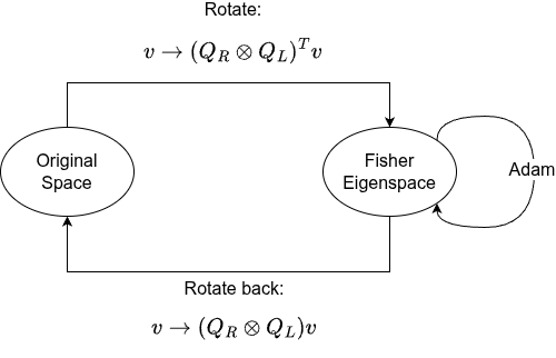
<p>SOAP then performs an Adam-like update in Shampoo’s eigenbasis:</p>

<ul>
  <li>Accumulate momentum $M$.</li>
  <li>Rotate both momentum $M$ and gradient $G$ to the Shampoo eigenbasis.</li>
  <li>Accumulate the second moment $\Sigma^*$ in that eigenbasis.</li>
  <li>Apply Adam-style normalization in the eigenbasis.</li>
  <li>Rotate the update back to the original parameter space.</li>
</ul>

<figure>
  <img src="/assets/images/fisher-optimizers/SOAP.png" alt="Scheme of SOAP update" style="width: min(520px, 100%); display: block; margin: 0 auto;" />
  <figcaption>Figure 1. Scheme of the SOAP update.</figcaption>
</figure>

<p>SOAP also avoids expensive repeated eigendecomposition. It uses randomized SVD-style iterations</p>

\[Q_t\gets \mathrm{QR}(AQ_{t-1}),\]

<p>which converge to the eigenvectors of $A$ under standard assumptions. If eigenvectors change slowly, one QR iteration every $k$ steps is often enough.</p>

<div class="framed algorithm-block">

  <p><strong>SOAP for a linear layer</strong></p>

  <ol>
    <li>Estimate $G_t\gets\nabla_W\mathcal{L}$.</li>
    <li>Update momentum $M_t\gets\beta_1M_{t-1}+(1-\beta_1)G_t$.</li>
    <li>Accumulate $L_t\gets\beta_2L_{t-1}+(1-\beta_2)G_tG_t^T$.</li>
    <li>Accumulate $R_t\gets\beta_2R_{t-1}+(1-\beta_2)G_t^TG_t$.</li>
    <li>Every $k$ steps, improve eigenvectors:</li>
  </ol>

\[Q_L\gets\mathrm{QR}(L_tQ_L),
\qquad
Q_R\gets\mathrm{QR}(R_tQ_R).\]

  <ol>
    <li>Rotate:</li>
  </ol>

\[\widetilde{G}_t\gets Q_L^TG_tQ_R,
\qquad
\widetilde{M}_t\gets Q_L^TM_tQ_R.\]

  <ol>
    <li>Accumulate eigenbasis second moment:</li>
  </ol>

\[\widetilde{V}_t
\gets
\beta_2\widetilde{V}_{t-1}
+
(1-\beta_2)(\widetilde{G}_t\odot\widetilde{G}_t).\]

  <ol>
    <li>Apply Adam in the eigenbasis and rotate back:</li>
  </ol>

\[\widetilde{U}_t
\gets
\frac{\widetilde{M}_t}{\sqrt{\widetilde{V}_t}+\varepsilon},
\qquad
U_t\gets Q_L\widetilde{U}_tQ_R^T.\]

  <ol>
    <li>Update $W_t\gets W_{t-1}-\eta U_t$.</li>
  </ol>

</div>

<h2 id="muon">Muon</h2>

<p>Bernstein observed that if Shampoo does not accumulate preconditioning matrices, equivalently $\beta_2=0$, then the update becomes [<a href="#bernstein2024old">Bernstein 2024</a>]:</p>

\[(GG^T)^{-1/4}G(G^TG)^{-1/4}.\]

<p>If $G=U\Sigma V^T$ is an SVD, the update reduces to</p>

\[UV^T,\]

<p>which is the matrix sign or polar factor [<a href="#higham2008functions">Higham 2008</a>]. This object can be interpreted as:</p>

<ul>
  <li>Orthogonalization:</li>
</ul>

\[UV^T
=
\operatorname*{argmin}_{QQ^T=I_n}
\|G-Q\|^2
\qquad
(D_{\mathrm{out}}\le D_{\mathrm{in}}).\]

<ul>
  <li>Steepest descent under a spectral-norm constraint:</li>
</ul>

\[UV^T
=
\operatorname*{argmax}_{\|H\|_2=1}
\langle G,H\rangle_F.\]

<p>Muon, short for Momentum Orthogonalized with Newton-Schulz, builds on this idea [<a href="#jordan2024muon">Jordan et al. 2024</a>]. Subsequent work studied how to scale Muon to large language model training [<a href="#liu2025muon">Liu et al. 2025</a>].</p>

<div class="framed algorithm-block">

  <p><strong>Muon for a linear layer (Moonlight lr scaling)</strong></p>

  <ol>
    <li>Estimate $G_t\gets\nabla_W\mathcal{L}(W_t)\in\mathbb{R}^{m\times n}$.</li>
    <li>Accumulate momentum $M_t\gets\beta M_{t-1}+G_t$.</li>
    <li>Use Nesterov momentum $\widehat{M}_t\gets\beta M_t+G_t$.</li>
    <li>Orthogonalize:</li>
  </ol>

\[U_t
\gets
\mathrm{NS5}(\widehat{M}_t)
\quad\text{if }m\le n,
\qquad
U_t
\gets
\mathrm{NS5}(\widehat{M}_t^T)^T
\quad\text{otherwise}.\]

  <ol>
    <li>Update</li>
  </ol>

\[W_{t+1}
\gets
W_t
-
0.2\,\eta\,\max(m,n)\,U_t.\]

</div>

<p>Here $\mathrm{NS5}$ denotes five Newton-Schulz iterations for approximate orthogonalization. This line of work is still developing, with variants such as Polar Express [<a href="#amsel2025polar">Amsel et al. 2025</a>] and Gram Newton-Schulz [<a href="#gramnewtonschulz">Zhang et al. 2026</a>]. Muon is currently a practical optimizer for LLM linear layers and is increasingly used as an AdamW alternative.</p>

<h2 id="experiments">Experiments</h2>

<h3 id="fisher-matrix-visualization">Fisher Matrix Visualization</h3>

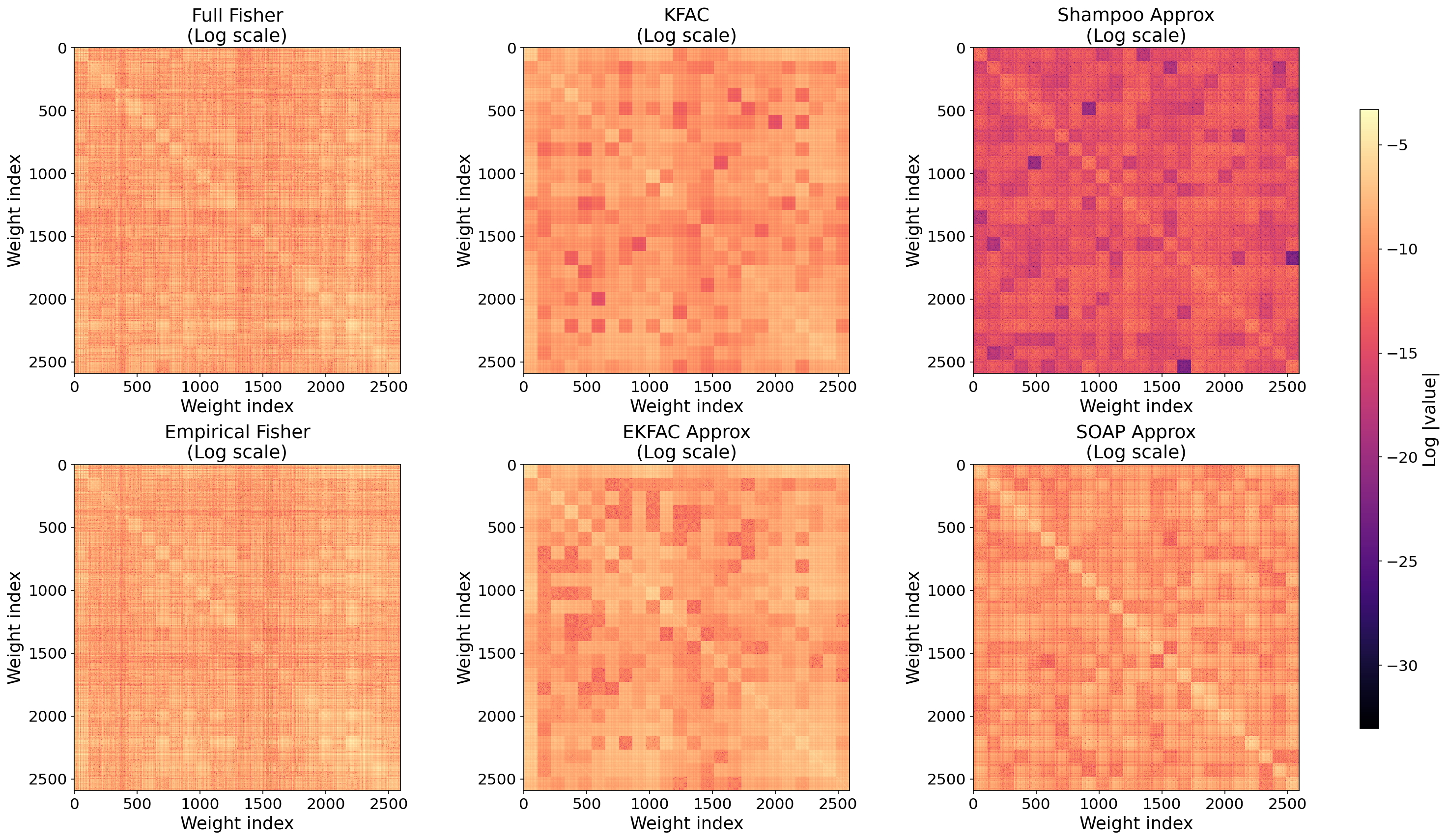
<p>The first experiment visualizes Fisher matrices for a small MNIST CNN with roughly 3800 parameters. Fisher approximations were computed after the 10th epoch, when the model was already well fitted.</p>

<p>Figure 2 shows six matrices using logarithms of absolute values. The first row contains the true Fisher (<a href="#eq-truefisher">Eq. 1</a>), KFAC (<a href="#eq-kfac-fisher">Eq. 4</a>), and Shampoo (<a href="#eq-shampoo-fisher">Eq. 6</a>). The second row contains the empirical Fisher (<a href="#eq-empiricalfisher">Eq. 2</a>), EKFAC (<a href="#eq-ekfac-fisher">Eq. 5</a>), and SOAP.</p>

<figure>
  <img src="/assets/images/fisher-optimizers/all-fisher-vis.png" alt="Visualization of true Fisher, KFAC, Shampoo, empirical Fisher, EKFAC, and SOAP approximations" style="width: 100%; display: block; margin: 0 auto;" />
  <figcaption>Figure 2. Visualization of six Fisher matrix approximations. First row: true Fisher, KFAC, Shampoo. Second row: empirical Fisher, EKFAC, SOAP.</figcaption>
</figure>

<p>The empirical Fisher is visually close to the true Fisher. This is plausible because the model is already well fitted and the model distribution is close to the data distribution. The small number of classes also helps. For LLM-like tasks with large vocabularies, the true Fisher can differ much more from the empirical Fisher.</p>

<p>KFAC and Shampoo show visible block structure. Shampoo has lower intensity, which may indicate poor eigenvalue approximation. SOAP and EKFAC improve these eigenvalues and smooth the block structure.</p>

<h3 id="llm-experiment">LLM Experiment</h3>

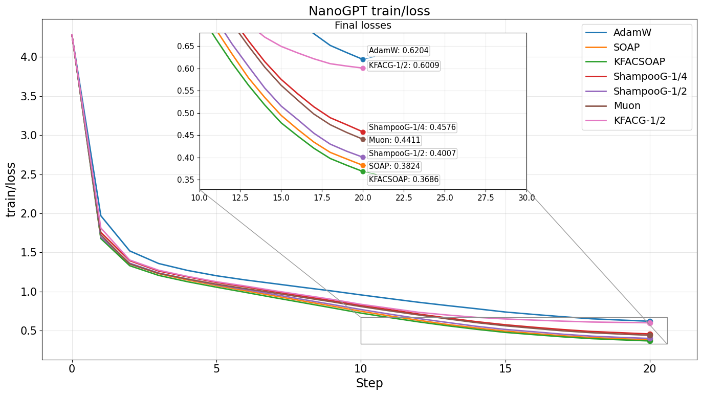
<p>The second experiment pretrains a small GPT-like model with roughly 10M parameters on Shakespeare-char. AdamW from Andrej Karpathy’s baseline was compared with Fisher-based optimizers. All optimizers that use SVD, meaning all except Muon and AdamW, use preconditioning every 10 steps.</p>

<figure>
  <img src="/assets/images/fisher-optimizers/exp.png" alt="Experimental comparison of AdamW, KFAC, Shampoo, SOAP, KFACSOAP, and Muon" style="width: 100%; display: block; margin: 0 auto;" />
  <figcaption>Figure 3. Experimental comparison of optimizers.</figcaption>
</figure>

<p>KFAC was run with power $-1/2$ instead of $-1$ because the latter was unstable and performed poorly. A suffix “G” indicates <strong>grafting</strong>, where the update is rescaled to have the Frobenius norm of the Adam update. This stabilizes the step size.</p>

<p>Shampoo was tested with powers $-1/4$, as in the original version, and $-1/2$, which corresponds more closely to inverting the Fisher instead of using its inverse square root. In this experiment, $-1/2$ performed significantly better. Muon performed similarly to Shampoo with power $-1/4$, but was substantially faster.</p>

<p>SOAP performed best among the considered optimizers. KFACSOAP is a SOAP modification where eigenvectors are computed using the KFAC approximation from <a href="#eq-kfac-fisher">Eq. 4</a> rather than the Shampoo approximation. It outperformed original SOAP in this experiment, suggesting that the KFAC approximation can be more accurate than Shampoo’s approximation in this setting.</p>

<p>Overall, SOAP-style optimizers performed best, supporting the idea that running Adam in an approximate Fisher eigenbasis is a strong practical recipe.</p>

<h2 id="conclusion">Conclusion</h2>

<p>Fisher-based optimizers can be viewed as attempts to approximate natural-gradient preconditioning in ways that fit modern neural networks. KFAC and EKFAC use activation and output-gradient statistics. Shampoo and SOAP use gradient-matrix structure. Muon can be understood as an efficient orthogonalized update arising from a limiting Shampoo-like view.</p>

<p>The experiments here suggest that SOAP-based methods are the most sample-efficient among the tested optimizers. A promising direction is improving eigenvector approximations. In the Shakespeare-char experiment, a KFAC-style eigenbasis worked better than Shampoo’s eigenbasis, which suggests that the choice of structured Fisher approximation still matters.</p>

<h2 id="references">References</h2>

<p><span id="amari1993backpropagation"></span>
Amari, S. (1993). <a href="https://doi.org/10.1016/0925-2312(93)90006-O">Backpropagation and stochastic gradient descent method</a>. <em>Neurocomputing</em>, 5(4-5), 185-196.</p>

<p><span id="kingma2014adam"></span>
Kingma, D. P., and Ba, J. (2014). <a href="https://arxiv.org/abs/1412.6980">Adam: A Method for Stochastic Optimization</a>. <em>arXiv:1412.6980</em>.</p>

<p><span id="amari2000methods"></span>
Amari, S., and Nagaoka, H. (2000). <a href="https://doi.org/10.1090/mmono/191"><em>Methods of Information Geometry</em></a>. American Mathematical Society.</p>

<p><span id="amari1998natural"></span>
Amari, S. (1998). <a href="https://doi.org/10.1162/089976698300017746">Natural gradient works efficiently in learning</a>. <em>Neural Computation</em>, 10(2), 251-276.</p>

<p><span id="martens2015optimizing"></span>
Martens, J., and Grosse, R. (2015). <a href="https://arxiv.org/abs/1503.05671">Optimizing Neural Networks with Kronecker-factored Approximate Curvature</a>. <em>ICML</em>.</p>

<p><span id="george2018fast"></span>
George, T., Laurent, C., Bouthillier, X., Ballas, N., and Vincent, P. (2018). <a href="https://proceedings.neurips.cc/paper/2018/hash/48000647b315f6f00f913caa757a70b3-Abstract.html">Fast Approximate Natural Gradient Descent in a Kronecker-factored Eigenbasis</a>. <em>NeurIPS</em>.</p>

<p><span id="gupta2018shampoo"></span>
Gupta, V., Koren, T., and Singer, Y. (2018). <a href="https://research.google/pubs/shampoo-preconditioned-stochastic-tensor-optimization/">Shampoo: Preconditioned Stochastic Tensor Optimization</a>. <em>ICML</em>.</p>

<p><span id="vyas2024soap"></span>
Vyas, N., Morwani, D., Zhao, R., Kwun, M., Shapira, I., Brandfonbrener, D., Janson, L., and Kakade, S. (2024). <a href="https://arxiv.org/abs/2409.11321">SOAP: Improving and Stabilizing Shampoo using Adam</a>. <em>arXiv:2409.11321</em>.</p>

<p><span id="bernstein2024old"></span>
Bernstein, J., and Newhouse, L. (2024). <a href="https://arxiv.org/abs/2409.20325">Old Optimizer, New Norm: An Anthology</a>. <em>arXiv:2409.20325</em>.</p>

<p><span id="higham2008functions"></span>
Higham, N. J. (2008). <a href="https://epubs.siam.org/doi/book/10.1137/1.9780898717778"><em>Functions of Matrices: Theory and Computation</em></a>. SIAM.</p>

<p><span id="jordan2024muon"></span>
Jordan, K., Jin, Y., Boza, V., You, J., Cesista, F., Newhouse, L., and Bernstein, J. (2024). <a href="https://kellerjordan.github.io/posts/muon/">Muon: An optimizer for hidden layers in neural networks</a>. Blog post.</p>

<p><span id="liu2025muon"></span>
Liu, J., Su, J., Yao, X., Jiang, Z., Lai, G., Du, Y., Qin, Y., Xu, W., Lu, E., Yan, J., Chen, Y., Zheng, H., Liu, Y., Liu, S., Yin, B., He, W., Zhu, H., Wang, Y., Wang, J., Dong, M., Zhang, Z., Kang, Y., Zhang, H., Xu, X., Zhang, Y., Wu, Y., Zhou, X., and Yang, Z. (2025). <a href="https://arxiv.org/abs/2502.16982">Muon is Scalable for LLM Training</a>. <em>arXiv:2502.16982</em>.</p>

<p><span id="amsel2025polar"></span>
Amsel, N., Persson, D., Musco, C., and Gower, R. M. (2025). <a href="https://arxiv.org/abs/2505.16932">The Polar Express: Optimal Matrix Sign Methods and Their Application to the Muon Algorithm</a>. <em>arXiv:2505.16932</em>.</p>

<p><span id="gramnewtonschulz"></span>
Zhang, J., Amsel, N., Chen, B., and Dao, T. (2026). <a href="https://dao-lab.ai/blog/2026/gram-newton-schulz/">Gram Newton-Schulz: A Fast, Hardware-Aware Newton-Schulz Algorithm for Muon</a>. Blog post and implementation note.</p>]]></content><author><name></name></author><category term="notes" /><summary type="html"><![CDATA[This post summarizes the natural-gradient view of deep learning optimization and reviews practical Fisher-based approximations for linear layers in chronological order. The central question is how methods such as KFAC, EKFAC, Shampoo and SOAP make structured preconditioning cheap enough to use in neural networks.]]></summary></entry><entry><title type="html">Properties of the Fisher Information Matrix</title><link href="https://fullfix.github.io/notes/2026/04/18/fisher-matrix-properties.html" rel="alternate" type="text/html" title="Properties of the Fisher Information Matrix" /><published>2026-04-18T00:00:00+00:00</published><updated>2026-04-18T00:00:00+00:00</updated><id>https://fullfix.github.io/notes/2026/04/18/fisher-matrix-properties</id><content type="html" xml:base="https://fullfix.github.io/notes/2026/04/18/fisher-matrix-properties.html"><![CDATA[<p>This post introduces the Fisher Information Matrix and develops its main statistical and geometric properties. It concludes with a short discussion of what Fisher singularity means and how it arises in overparameterized models.</p>

<!--more-->

<h2 id="statistical-interpretation">Statistical Interpretation</h2>

<p>We start by introducing Fisher Information Matrix and describing its statistical properties which help understand the intuition behind the word “information” in the name.</p>

<p>First, let us define the set of distributions that we will be working with. We understand distribution $p_{\theta}: \mathbb{R}^{d} \to \mathbb{R}$ as a map such that $\int p_{\theta}(x)\,dx = 1$ and $p_{\theta}(x) \ge 0$ for all $x$. Each $\theta \in \Theta \subset \mathbb{R}^{n}$ defines its own distribution and is called parameter. The open set $\Theta$ is called a parameter space. The set of distributions that are formed by all possible parameters is called a statistical model with dimension $n$:</p>

\[S := \{\, p_\theta \mid \theta \in \Theta \,\}.\]

<p>Strictly speaking, the mapping $\theta \leftrightarrow p_\theta$ should be bijective and $\Theta$ should be an open set in $\mathbb{R}^n$ for the correct definition of the statistical model. However, due to the common case of overparameterization in neural networks, we omit this requirement in the section on singularity, where we analyze the connection between overparameterization and Fisher matrix.</p>

<p>We will make the following assumptions about the statistical model and the distributions:</p>

\[\forall x\in\mathbb X,\quad \theta\mapsto p_\theta(x)\in C^\infty(\Theta)\]

\[\operatorname{supp}(p_\theta)=\mathbb X \quad \text{for all } \theta\in\Theta\]

\[\text{Regularity for } \frac{\partial }{\partial \theta }p_\theta(x),\ s_\theta(x),\ s_\theta(x)s_\theta(x)^T,\ \frac{\partial^2}{\partial\theta^2}\log p_{\theta}(x)\]

\[\mathbb{E}_\theta \left[\left|s_\theta s_\theta^T\right|\right] &lt; \infty\]

<p>Here we denote</p>

\[s_\theta(x) := \frac{\partial}{\partial \theta}\log p_\theta(x)\]

<p>and call it a <strong>score function</strong>.</p>

<p>The first assumption is classical for statistical models. We typically require sufficiently smooth dependence on $\theta$ for derivatives to exist.</p>

<p>The second assumption implies that the support of the distribution does not depend on $\theta$. It is an important requirement for interchanging $\frac{\partial}{\partial \theta}$ and $\int$ and filters out distributions such as Uniform $U[0, \theta]$.</p>

<p>The third assumption requires existence of the (element-wise) integrals and ability to interchange $\frac{\partial}{\partial \theta}$ and $\int$. More strictly, for a function
$f_\theta(x) \in { \frac{\partial }{\partial \theta }p_\theta(x), \ldots }$ we need:</p>

\[\begin{aligned}
\forall \theta_0\in\Theta,\ &amp;\exists \text{ a neighborhood } U \ni \theta_0,\ \exists g\in L^1(\mathbb X) \\
&amp;\text{such that }
|f_\theta(x)|\le g(x)
\quad \forall \theta\in U,\ \forall x\in\mathbb X.
\end{aligned}\]

<p>The fourth assumption is required for the existence of the Fisher Information Matrix, which will be introduced later.</p>

<p>The score function $s_\theta(x)$ plays an important role in machine learning. Using chain rule, we can express density derivative in terms of the score:</p>

\[s_\theta(x)=\frac{\partial}{\partial \theta}\log p_\theta(x)
= \frac{1}{p_\theta(x)}\frac{\partial}{\partial \theta}p_\theta(x)
\implies
\frac{\partial}{\partial \theta}p_\theta(x) = s_\theta(x)p_\theta(x)\]

<p>The main property of the score function is having zero mean:</p>

\[\mathbb{E}_\theta [s_\theta]
=
\int s_\theta(x)p_\theta(x)\,dx
=
\int \frac{\partial}{\partial \theta}p_\theta(x)\,dx
\overset{\text{regularity}}{=}
\frac{\partial}{\partial \theta} \int p_\theta(x)\,dx
=
\frac{\partial}{\partial \theta} 1
=
0\]

<p>Let us define the Fisher Information Matrix, the main object of the current document. We will also call it Fisher matrix or just Fisher.</p>

\[F(\theta) := \mathbb{E}_\theta \left[s_\theta s_\theta^T\right] = \operatorname{Cov}(s_\theta) \succeq 0\]

<p>Fisher matrix is also the covariance matrix of the score function due to zero mean of the latter. By definition, it is positive semidefinite.</p>

<div class="framed">

  <div class="statementinner">

    <p><strong>Statement.</strong></p>

\[F(\theta)
=
\mathbb{E}_\theta\left[s_\theta s_\theta ^T\right]
=
\mathbb{E}_\theta \left[\frac{\partial^2}{\partial \theta^2}(-\log p_\theta )\right]\]

  </div>

</div>

<h4 id="proof">Proof</h4>

<p>Using the score property:</p>

\[\mathbb{E}_\theta \left[s_\theta \right] = \int s_\theta(x)p_\theta(x)\,dx = 0\]

<p>Differentiating by $\theta$ on both sides (and using regularity) gives:</p>

\[\int \left[
\left(\frac{\partial}{\partial \theta}s_\theta(x)\right) p_\theta(x)
+
s_\theta(x)\left(\frac{\partial}{\partial \theta}p_\theta(x)\right)^T
\right]dx = 0\]

<p>Rewriting the score by the definition on the left side and substituting the identity
$\frac{\partial}{\partial \theta}p_\theta(x) = s_\theta(x)p_\theta(x)$
on the right side proves the statement.</p>

<hr />

<p>Next, we would like to discuss the connection of the Fisher matrix with sufficient statistics. By statistic we mean any smooth function $T: \mathbb{X} \to \mathbb{R}^m$. We assume sufficient smoothness $T(x) \in C^{\infty}(\mathbb{X})$. If we denote $X$ as a random variable with distribution $p_\theta(x)$, then we denote $T(X)$ as a random variable with distribution:</p>

\[q_\theta (t)
=
\int \delta (T(x) - t) p_\theta(x)\,dx
=
\mathbb{E}_\theta \bigl[\delta (T(x) - t)\bigr]\]

<p>We call $T(X)$ a sufficient statistic if $p_\theta (x) / q_\theta (T(x))$ does not depend on $\theta$, or in other words $p_\theta(x) = c(x)q_\theta(T(x))$. In fact, it is sufficient to find any positive function $g_\theta$, such that $p_\theta(x) = c(x)g_\theta(T(x))$. This equivalence is called factorization theorem. It can be easily proved with the following observation:</p>

\[q_\theta (t)
=
\int \delta(T(x) - t)\, c(x)g_\theta(T(x))\,dx
=
g_\theta(t)C(t)\]

<p>So we can rewrite factorization with any function $g_\theta$ as follows:</p>

\[p_\theta(x)
=
c(x)g_\theta(T(x))
=
\left(\frac{c(x)}{C(T(x))}\right)q_\theta(T(x))\]

<div class="framed">

  <div class="statementinner">

    <p><strong>Statement.</strong></p>

    <p>If $T(x)$ is a statistic for the statistical model ${ p_\theta }$ and we denote</p>

\[F(\theta) = \mathbb{E}_\theta \left[ s_\theta s_\theta^T \right],
\qquad
s_\theta(x) = \frac{\partial}{\partial \theta} \log p_\theta(x)\]

\[F_T(\theta) = \widetilde{\mathbb{E}}_\theta \left[ \widetilde{s}_\theta \widetilde{s}_\theta^T \right],
\qquad
\widetilde{s}_\theta(t) = \frac{\partial}{\partial \theta} \log q_\theta(t)\]

    <p>then $F(\theta) \succeq F_T(\theta)$, and equality holds if and only if $T$ is a sufficient statistic.</p>

  </div>

</div>

<h4 id="proof-1">Proof</h4>

<p>For any value $t$ of the statistic:</p>

\[q_\theta(t) = \int \delta (T(x) - t )p_\theta(x)\,dx\]

<p>Differentiate with respect to $\theta$:</p>

\[\frac{\partial}{\partial \theta} q_\theta(t)
=
\int \delta(T(x) - t) p_\theta(x)s_\theta(x)\,dx\]

<p>Now, dividing both sides by $q_\theta(t)$ and using the definition of conditional expectation, we get:</p>

\[\widetilde{s}_\theta(t) = \mathbb{E}_\theta\left[s_\theta \mid T = t \right]\]

<p>For any fixed $t$:</p>

\[\operatorname{Cov}(s_\theta \mid T=t)
:=
\mathbb{E}_\theta[s_\theta s_\theta^T \mid T = t]
-
\mathbb{E}_\theta[s_\theta \mid T = t]\mathbb{E}_\theta[s_\theta \mid T = t]^T
\succeq 0\]

<p>Now we take expectation with respect to $T$:</p>

\[\begin{aligned}
\widetilde{\mathbb{E}}\left[\mathbb{E}_\theta\left[s_\theta s_\theta^T \mid T \right] \right]
&amp;=
\int
\frac{
\int \delta(T(x)-t)\, s_\theta(x)s_\theta(x)^T p_\theta(x)\,dx
}{
q_\theta(t)
}
q_\theta(t)\,dt
\\
&amp;=
\int
s_\theta(x)s_\theta(x)^T p_\theta(x)
\left(
\int \delta(T(x)-t)\,dt
\right) dx
\\
&amp;=
\int s_\theta(x)s_\theta(x)^T p_\theta(x)\,dx
\\
&amp;=
\mathbb{E}_\theta\left[s_\theta s_\theta^T\right]
\end{aligned}\]

<p>After integrating with positive factor $q_\theta(t)$, the covariance matrix still remains positive semidefinite. We also substitute $\widetilde{s}_\theta(t)$ for the second term:</p>

\[\mathbb{E}_\theta \left[s_\theta s_\theta^T \right]
-
\widetilde{\mathbb{E}}_\theta\left[\widetilde{s}_\theta \widetilde{s}_\theta^T \right]
\succeq 0\]

<p>Hence</p>

\[F(\theta) - F_T(\theta) \succeq 0\]

<p>Now note that equality to zero means that the expectation of a positive semidefinite matrix is zero, thus equivalently for all $t$:</p>

\[\operatorname{Cov}(s_\theta \mid T = t) = 0\]

<p>Equivalently, after fixing $T = t$, $s_\theta(x)$ becomes a constant. We can express this as:</p>

\[s_\theta(x)
=
\frac{\partial}{\partial \theta}\log p_\theta(x)
=
a_\theta(T(x))\]

<p>For fixed $t$ and $x$ with $T(x) = t$, we can differentiate $a_\theta$ to obtain:</p>

\[\frac{\partial}{\partial \theta_j} (a_\theta(T(x)))_i
=
\frac{\partial^2}{\partial \theta_i \partial \theta_j}\log p_\theta(x)
=
\frac{\partial}{\partial \theta_i}(a_\theta(T(x)))_j\]

<p>So $a_\theta$ can be expressed as a gradient of some scalar function. Reparameterize:</p>

\[a_\theta(t) = \frac{\partial}{\partial \theta}\log g_\theta(t)\]

<p>Then</p>

\[\frac{\partial}{\partial \theta}\left[\log p_\theta(x) - \log g_\theta(T(x)) \right]
=
\frac{\partial}{\partial\theta}\log \frac{p_\theta(x)}{g_\theta(T(x))}
=
0\]

<p>This results in $p_\theta(x) = c(x) g_\theta(T(x))$ and completes the proof by the factorization theorem.</p>

<hr />

<p>This theorem shows us an intuitive interpretation of Fisher matrix: when performing any transformation $T(x)$, we lose “information” about the parameter $\theta$. However, when $T(x)$ is a sufficient statistic, it keeps all “information” about $\theta$.</p>

<p>We call a statistic $T: \mathbb{X} \to \mathbb{R}^n$ <strong>locally unbiased</strong> at point $\theta_0$ if for any $\theta$ from some neighborhood of $\theta_0$ we have:</p>

\[\mathbb{E}_\theta \left[T\right] = \theta\]

<p>Now comes the famous Cramér–Rao inequality which provides a lower bound on the estimation error for an unbiased estimator.</p>

<div class="framed">

  <div class="statementinner">

    <p><strong>Statement (Cramér–Rao inequality).</strong></p>

    <p>Let ${p_\theta }$ be a statistical model and $T: \mathbb{X} \to \mathbb{R}^n$ be a locally unbiased estimator for some parameter $\theta \in \mathbb{R}^n$. Denote:</p>

\[F(\theta) = \mathbb{E}_\theta\left[ s_\theta s_\theta^T \right] \succ 0,
\qquad
s_\theta(x) = \frac{\partial}{\partial \theta}\log p_\theta(x)\]

    <p>Then:</p>

\[\operatorname{Cov}_\theta(T) \succeq F(\theta)^{-1}\]

  </div>

</div>

<h4 id="proof-2">Proof</h4>

<p>It is easy to show that for a locally unbiased estimator which satisfies
$\mathbb{E}_{\widetilde{\theta}}\left[T\right] = \widetilde{\theta}$
for some neighborhood of $\theta$:</p>

\[\frac{\partial}{\partial \theta} \mathbb{E}_\theta \left[T\right]
=
\mathbb{E}_\theta \left[ Ts_\theta \right]
=
I_n\]

<p>Using the score function property $\mathbb{E}<em>\theta s</em>\theta = 0$, we can subtract
$0 = \theta \mathbb{E}<em>\theta s</em>\theta$:</p>

\[\mathbb{E}_\theta \left[ (T - \theta)s_{\theta}\right]
=
I_n
=
\operatorname{Cov}(T - \theta, s_\theta )\]

<p>If we consider the stacked random vector
$\begin{bmatrix} T - \theta \ s_\theta \end{bmatrix}$
and take its covariance matrix, we get:</p>

\[\begin{bmatrix}
\operatorname{Cov}(T) &amp; I_n \\
I_n &amp; F(\theta)
\end{bmatrix} \succeq 0\]

<p>Schur complement with respect to $F(\theta)$ gives:</p>

\[\operatorname{Cov}(T) - I_n F(\theta)^{-1}I_n \succeq 0\]

<p>which proves the theorem.</p>

<hr />

<p>Cramér–Rao inequality allows us to interpret Fisher matrix as a lower bound on the uncertainty of estimation. If $F(\theta)$ has eigenvalues close to $0$, its inverse has large eigenvalues and therefore estimation is very poor. On the contrary, large eigenvalues of $F(\theta)$ provide a lot of “information” about the parameter for the estimator. The estimators that achieve equality in Cramér–Rao are called efficient.</p>

<p>Next property allows us to understand how Fisher behaves when distribution consists of independent variables and is factorized by them.</p>

<div class="framed">

  <div class="statementinner">

    <p><strong>Statement.</strong></p>

    <p>Let $X_1, X_2$ be independent random variables with distributions $p_{\theta_1}(x), p_{\theta_2}(x)$. Denote $\theta = [\theta_1, \theta_2]$ as stacked parameter. Denote $F_1(\theta_1), F_2(\theta_2)$ as Fisher matrices of individual distributions, and $F(\theta)$ as Fisher matrix of the joint distribution
$p_\theta(x) = p_{\theta_1}(x_1)p_{\theta_2}(x_2)$.
Then joint Fisher matrix is block-diagonal:</p>

\[F(\theta) =
\begin{bmatrix}
F_1(\theta_1) &amp; 0 \\
0 &amp; F_2(\theta_2)
\end{bmatrix}\]

  </div>

</div>

<h4 id="proof-3">Proof</h4>

<p>When considering full parameter $\theta$, we have:</p>

\[s_{\theta}(x)
=
\frac{\partial}{\partial \theta}\log \bigl(p_{\theta_1}(x_1)p_{\theta_2}(x_2)\bigr)
=
\begin{bmatrix}
s_{\theta_1}(x_1) \\
0
\end{bmatrix}
+
\begin{bmatrix}
0 \\
s_{\theta_2}(x_2)
\end{bmatrix}
=
\begin{bmatrix}
s_{\theta_1}(x_1) \\
s_{\theta_2}(x_2)
\end{bmatrix}\]

<p>Now, Fisher matrix has form:</p>

\[F(\theta)
=
\mathbb{E}_\theta
\begin{bmatrix}
s_{\theta_1}s_{\theta_1}^T &amp; s_{\theta_1} s_{\theta_2}^T \\
s_{\theta_2}s_{\theta_1}^T &amp; s_{\theta_2}s_{\theta_2}^T
\end{bmatrix}
=
\begin{bmatrix}
\mathbb{E}_\theta \left[ s_{\theta_1}s_{\theta_1}^T \right] &amp; 0 \\
0 &amp; \mathbb{E}_\theta \left[ s_{\theta_2}s_{\theta_2}^T \right]
\end{bmatrix}
=
\begin{bmatrix}
F_1(\theta_1) &amp; 0 \\
0 &amp; F_2(\theta_2)
\end{bmatrix}\]

<p>where off-block-diagonal entries vanish due to expectation factorization and the zero-mean property of the score function.</p>

<hr />

<p>So, independence of the parameters is nicely reflected in the Fisher matrix. The inverse implication, however, is generally false: block-diagonal Fisher matrix does not imply independence. Next, when all independent distributions depend on the same parameter, we also get a specific form of the joint Fisher matrix.</p>

<div class="framed">

  <div class="statementinner">

    <p><strong>Statement.</strong></p>

    <p>Let $X_1, \ldots, X_N$ be $N$ independent random variables with distributions
$p_{\eta_1}(x), \ldots, p_{\eta_N}(x)$, where $\eta_i = f_i(\theta)$ and $\theta$ is the shared parameter.
The joint distribution has form:</p>

\[p_\theta(x_1, \ldots, x_N) = p_{\eta_1(\theta)}(x_1) \cdots p_{\eta_N(\theta)}(x_N)\]

    <p>Let us denote $F_1(\theta), \ldots, F_N(\theta)$ as Fisher matrices of individual distributions, and $F(\theta)$ as Fisher of the joint distribution. Then:</p>

\[F(\theta) = F_1(\theta) + \cdots + F_N(\theta)\]

  </div>

</div>

<h4 id="proof-4">Proof</h4>

<p>Score function of the joint distribution takes form:</p>

\[s(x_1, \ldots, x_N)
=
\frac{\partial}{\partial \theta}\log p_\theta(x_1, \ldots, x_N)
=
\frac{\partial}{\partial \theta} \sum_{i=1}^N \log p_{\eta_i(\theta)}(x_i)
=
\sum_{i=1}^N s_{\theta}^{(i)}(x_i)\]

<p>where</p>

\[s_\theta^{(i)}(x_i) := \frac{\partial}{\partial \theta}\log p_{\eta_i(\theta)}(x_i)\]

<p>Then:</p>

\[F(\theta)
=
\mathbb{E}_{\theta}\left[ss^T\right]
=
\sum_{i=1}^N \mathbb{E}_{\theta}\left[ s_{\theta}^{(i)}\left(s_{\theta}^{(i)}\right)^T \right]
+
\sum_{i \ne j} \mathbb{E}_{\theta}\left[s_{\theta}^{(i)}\right]\mathbb{E}_{\theta}\left[s_{\theta}^{(j)} \right]^T
=
\sum_{i=1}^N F_{i}(\theta)\]

<p>where the second term with $i \ne j$ vanishes due to the zero-mean property of the score function.</p>

<hr />

<p>Intuitively, this means that when independent variables are combined, their “information” is added.</p>

<p>When considering estimation with $N$ independent samples from distribution $p_{\theta}$ with Fisher matrix $F(\theta)$, we get the simplification:</p>

\[F_{(N)}(\theta) = N F(\theta)\]

<p>Now, due to Cramér–Rao inequality, a locally unbiased estimator
$T(x_1, \ldots, x_N)$
for the joint distribution
$p(x_1)\cdots p(x_N)$
satisfies:</p>

\[\operatorname{Cov}_\theta(T) \succeq \frac{F(\theta)^{-1}}{N}\]

<p>This provides a bound on the convergence of a locally unbiased estimator when $N \to \infty$.</p>

<h2 id="fisher-metric">Fisher Metric</h2>

<p>Let us introduce the inner product between parameter changes
$d\theta_1, d\theta_2 \in \mathbb{R}^n$
induced by the Fisher matrix:</p>

\[\langle d\theta_1, d\theta_2 \rangle_F := d\theta_2^T F d\theta_1\]

<p>Let us call $\langle \cdot , \cdot \rangle_F$ the Fisher metric. Obviously, it is not a metric in the usual elementary sense. However, it has a connection to differential geometry.</p>

<p>One of the main properties of the Fisher metric is its invariance with respect to reparameterization. For theoretical rigor, we only consider diffeomorphisms. By diffeomorphism we mean a $C^1$ map between $\mathbb{R}^n$ and $\mathbb{R}^n$ which is bijective and whose inverse is also $C^1$.</p>

<div class="framed">

  <div class="statementinner">

    <p><strong>Statement.</strong></p>

    <p>Fisher metric is invariant under any diffeomorphism $\theta(\eta)$ with Jacobian</p>

\[J(\eta) = \frac{\partial \theta}{\partial \eta}.\]

  </div>

</div>

<h4 id="proof-5">Proof</h4>

<p>Let</p>

\[J(\eta) := \frac{\partial}{\partial \eta}\theta(\eta)\]

<p>be the Jacobian of the reparameterization. By the chain rule:</p>

\[\frac{\partial}{\partial \eta}\log p_{\theta(\eta)}(x)
=
J(\eta)^T \frac{\partial}{\partial \theta } \log p_\theta (x),
\qquad
s_\eta (x) = J(\eta)^T s_{\theta (\eta)}(x)\]

<p>Fisher matrix in the new coordinates $\eta$ can be written as:</p>

\[F_\eta (\eta)
=
\mathbb{E}\left[ s_\eta s_\eta^T \right]
=
\mathbb{E} \left[ J(\eta)^T s_{\theta(\eta)}s_{\theta(\eta)}^T J(\eta)  \right]
=
J(\eta)^T F_\theta (\theta(\eta)) J(\eta)\]

<p>Now let $d\eta_1, d\eta_2$ be infinitesimal parameter changes in $\eta$ space. Then:</p>

\[d\theta_1 = J(\eta)d\eta_1,
\qquad
d\theta_2 = J(\eta)d\eta_2\]

<p>Hence:</p>

\[\langle d\eta_1,d\eta_2\rangle_{F_\eta}
=
d\eta_1^T F_\eta(\eta)d\eta_2
=
d\eta_1^T J(\eta)^T F_\theta(\theta(\eta)) J(\eta)d\eta_2
=
d\theta_1^T F_\theta(\theta(\eta)) d\theta_2
=
\langle d\theta_1,d\theta_2\rangle_{F_\theta}\]

<hr />

<p>So, Fisher metric does not depend on the particular choice of parameterization, making it an effective inner product between infinitesimal distribution changes. In fact, when $F \succ 0$, Fisher metric is a Riemannian metric on the statistical manifold.</p>

<p>Fisher metric has connections to the KL divergence</p>

\[KL(p_1 \,\|\, p_2) := \mathbb{E}_1\log \frac{p_1}{p_2}.\]

<p>Consider a point $\theta \in \mathbb{R}^n$ and a small parameter change $\Delta \theta \in \mathbb{R}^n$. KL divergence between $\theta$ and $\theta + \Delta \theta$ is:</p>

\[K(\theta, \theta + \Delta \theta)
:=
KL(p_{\theta} \,\|\, p_{\theta + \Delta \theta})
=
\mathbb{E}_\theta \left[ \log \frac{p_\theta}{p_{\theta + \Delta \theta}} \right]\]

<p>We would like to write the Taylor expansion up to second order. The first term in KL divergence is fixed, and we differentiate with respect to the second term. For that, we compute:</p>

\[\frac{\partial }{\partial \eta } K(\theta, \eta)
=
\frac{\partial }{\partial \eta } \mathbb{E}_\theta \left[ \log p_\theta - \log p_\eta  \right]
=
-\mathbb{E}_\theta \left[ \frac{\partial }{\partial \eta} \log p_\eta \right]
=
-\mathbb{E}_\theta \left[ s_\eta \right]\]

\[\frac{\partial^2}{\partial \eta ^2} K(\theta, \eta)
=
-\mathbb{E}_\theta \left[ \frac{\partial ^2}{\partial \eta^2}\log p_\eta  \right]\]

<p>The first derivative vanishes at point $\theta$ due to the zero-mean property of the score function. The second derivative becomes $F(\theta)$ by the identity proved earlier.</p>

<p>Thus:</p>

\[KL(p_\theta \,\|\, p_{\theta + \Delta \theta} )
=
\frac{1}{2}\Delta \theta^T F(\theta) \Delta \theta + O(\|\Delta \theta\|^3)
=
\frac{1}{2}\|\Delta \theta \|^2_F + O(\|\Delta \theta\|^3)\]

<p>where the norm $|\cdot |_F := \sqrt{\langle \cdot, \cdot \rangle_F}$ is induced by the Fisher metric.</p>

<p>So, Fisher metric provides a second-order approximation of the KL divergence. This makes it suitable for trust-region methods with KL constraint.</p>

<p>Next, let us derive an object closely related to the Fisher metric. We can view $\langle \cdot, \cdot \rangle_F$ as an ordinary Euclidean scalar product for transformed vectors:
$v \mapsto F^{1/2}v$.
The volume change induced by this transformation can be expressed with determinant
$\det(F^{1/2}) = \det(F)^{1/2}$.</p>

<p>Jeffreys prior is a prior distribution on parameters $\theta$ that assigns probability mass proportionally to “information volume”:</p>

\[\pi _J (\theta) \propto \sqrt{\det \left(F(\theta)\right)}\]

<p>Here, for correct definition, we consider the case where $F(\theta) \succ 0$ for all $\theta$.</p>

<div class="framed">

  <div class="statementinner">

    <p><strong>Statement.</strong></p>

    <p>Jeffreys prior is invariant under any diffeomorphism $\theta(\eta)$ with Jacobian</p>

\[J(\eta) = \frac{\partial \theta}{\partial \eta}.\]

  </div>

</div>

<h4 id="proof-6">Proof</h4>

<p>From the proof of Fisher metric invariance:</p>

\[s_\eta(x,\eta) = J(\eta)^T s_\theta(x,\theta),
\qquad
F_\eta(\eta) = J(\eta)^TF_\theta(\theta(\eta))J(\eta)\]

<p>Taking determinants, we obtain</p>

\[\det F_\eta(\eta)
=
\det(J^T F_\theta(\theta) J)
=
\det(J)^2 \det(F_\theta(\theta))\]

<p>hence</p>

\[\sqrt{\det F_\eta(\eta)} = |\det J(\eta)| \sqrt{\det F_\theta(\theta)}\]

<p>For reparameterization of the distribution, we know that:</p>

\[\pi^*_J(\eta) = |\det J(\eta)|\pi_J(\theta(\eta))\]

<p>Now it is easy to see that:</p>

\[\pi_J(\eta)
:=
\sqrt{\det F_\eta(\eta)}
=
|\det J(\eta)| \sqrt{\det F_\theta (\theta)}
=
|\det J(\eta)| \pi_J(\theta)
=
\pi^*_J(\eta)\]

<p>Thus, Jeffreys prior is invariant under smooth reparameterization.</p>

<h2 id="singularity-analysis">Singularity analysis</h2>

<p>Usually, statistics books consider the statistical model to always have positive definite Fisher matrix $F \succ 0$, however we would like to provide interpretation of its singularity.</p>

<p>First, let us slightly weaken the definition of the statistical model: $\Theta$ is a set in $\mathbb{R}^n$ (not necessarily open), and the map $\theta \mapsto p_\theta$ at each point $x$ does not have to be bijective, though it is still $C^1(\Theta)$.</p>

<p>Let us call the statistical model <strong>locally overparameterized</strong> at point $\theta \in \Theta$ if there exists a direction $v \in \mathbb{R}^n$ that does not change a distribution in first order:</p>

\[\left. \frac{d}{dt}p_{\theta + tv}(x) \right|_{t=0} = 0
\quad \forall x \in \mathbb{X}\]

<p>We can equivalently express this in terms of the score function using directional derivative:</p>

\[\left. \frac{d}{dt}p_{\theta + tv}(x) \right|_{t=0} = 0
\iff
\left. \frac{d}{dt}\log p_{\theta + tv}(x) \right|_{t=0}
=
\frac{\partial \log p_\theta(x)}{\partial v}
=
\langle s_\theta(x), v \rangle
=
0\]

<div class="framed">

  <div class="statementinner">

    <p><strong>Statement (Criterion of singularity of the Fisher matrix).</strong></p>

    <p>Fisher matrix $F(\theta)$ is singular if and only if the model is locally overparameterized at point $\theta$.</p>

  </div>

</div>

<h4 id="proof-7">Proof</h4>

\[\langle Fv, v \rangle
=
\mathbb{E}\left[\langle s_\theta, v \rangle^2\right]
=
0
\iff
\langle s_\theta(x), v \rangle = 0 \quad \forall x
\iff
\text{the model is locally overparameterized at } \theta\]

<hr />

<p>This simple criterion allows us to intuitively understand that zero eigenvalues of the Fisher matrix correspond to directions that do not change the distribution locally. Hence, they do not contain any “information” about the distribution locally.</p>

<p>When strictly defining a statistical model, local overparameterization does not exist.</p>

<div class="framed">

  <div class="statementinner">

    <p><strong>Statement.</strong></p>

    <p>If $\Theta \subset \mathbb{R}^n$ and $\theta \leftrightarrow p_\theta$ is a diffeomorphism, then the model is not locally overparameterized at any point. Equivalently, $F(\theta) \succ 0$ for every $\theta \in \Theta$.</p>

  </div>

</div>

<h4 id="proof-8">Proof</h4>

<p>Fix any $\theta \in \Theta$. Suppose the model is locally overparameterized at $\theta$. Then there exists a nonzero direction $v \in \mathbb{R}^n$, $v \ne 0$, such that</p>

\[\left. \frac{d}{dt} p_{\theta + tv}(x) \right|_{t=0} = 0
\qquad \forall x \in \mathbb{X}\]

<p>Denote by $\Phi(\theta) = p_\theta$ the map from parameters to distributions. Since $\theta \leftrightarrow p_\theta$ is a diffeomorphism, it can never have any directional derivative equal to zero. Therefore,</p>

\[\left. \frac{d}{dt} p_{\theta + tv} \right|_{t=0}
=
\left. \frac{d}{dt} \Phi(\theta + tv) \right|_{t=0}
\ne 0\]

<p>which is a contradiction.</p>

<div class="framed">

  <div class="statementinner">

    <p><strong>Statement.</strong></p>

    <p>If $T(x)$ is locally unbiased at point $\theta_0$, then the statistical model is not locally overparameterized at point $\theta_0$.</p>

    <p>Equivalently, if the model is locally overparameterized at $\theta_0$, a locally unbiased estimator at $\theta_0$ does not exist.</p>

  </div>

</div>

<h4 id="proof-9">Proof</h4>

<p>Suppose $T(x)$ is a locally unbiased estimator at $\theta_0$ and also the model is locally overparameterized at $\theta_0$: there exists a direction $v \ne 0$ such that for all $x$,</p>

\[\left. \frac{d}{dt}p_{\theta + tv}(x) \right|_{t=0} = 0\]

<p>As the estimator is unbiased in some neighborhood of $\theta_0$, for sufficiently small $t$ we have:</p>

\[\mathbb{E}_\theta \left[T \right] = \theta,
\qquad
\mathbb{E}_{\theta + tv}\left[T\right] = \theta + tv\]

<p>This implies:</p>

\[\mathbb{E}_{\theta + tv}\left[T\right] - \mathbb{E}_\theta \left[T \right]
=
\int T(x)\left(p_{\theta + tv}(x) - p_\theta(x)\right)\,dx
=
tv\]

<p>Dividing by $t$ and taking the limit $t \to 0$:</p>

\[\int T(x)\left. \frac{d}{dt}p_{\theta + tv}(x) \right|_{t=0}dx
=
0
=
v\]

<p>This contradiction proves the statement.</p>

<hr />

<p>In neural networks, typically there is redundancy of parameters in a sense that model dimension can be reduced. The final statement of this section naturally explains the behavior of the Fisher matrix for such case.</p>

<div class="framed">

  <div class="statementinner">

    <p><strong>Statement.</strong></p>

    <p>Let</p>

\[\theta \in \Theta = \mathbb{R}^n \mapsto \eta(\theta) \in \Omega \subset \mathbb{R}^m\]

    <p>be a $C^1$ map with Jacobian</p>

\[J(\theta) := \frac{\partial}{\partial \theta}\eta(\theta) \in \mathbb{R}^{m \times n},
\qquad m &lt; n\]

    <p>where $\Omega$ is an open set. Suppose there is a bijection
$\eta(\theta) \leftrightarrow p_{\eta(\theta)}$
and $\eta(\theta) \mapsto p_{\eta(\theta)}(x)$ is $C^{\infty}$ for all $x \in \mathbb{X}$.
In other words, $p_{\eta(\theta)}$ is an $m$-dimensional statistical model in the strict sense.</p>

    <p>Then if we consider the $n$-dimensional parameterization
$\theta \mapsto p_\theta := p_{\eta(\theta)}$,
and define the $n \times n$ Fisher matrix</p>

\[F(\theta) := \mathbb{E}_\theta \left[s_\theta s_\theta^T \right],\]

    <p>the following holds:</p>

\[\operatorname{rank}(F(\theta)) = \operatorname{rank}(J(\theta)) \le m\]

    <p>In particular, when Jacobian $J(\theta)$ has full row rank $m$ for every $\theta$, Fisher matrix $F(\theta)$ always has rank $m$.</p>

  </div>

</div>

<h4 id="proof-10">Proof</h4>

<p>From the chain rule, similarly to the reparameterization formula, we have:</p>

\[F(\theta) = J(\theta)^T F_{\eta}(\eta(\theta))J(\theta)\]

<p>Because $\eta(\theta) \leftrightarrow p_{\eta(\theta)}$ is a diffeomorphism, the $m \times m$ Fisher matrix $F_{\eta}(\eta(\theta))$ is positive definite, and therefore has full rank $m$.</p>

<p>Now the following sequence of equivalences shows that
$\ker F(\theta) = \ker J(\theta)$
and therefore their ranks are equal:</p>

\[F(\theta)v = 0
\iff
\langle F(\theta)v, v\rangle = 0
\iff
\left\langle F_\eta(\eta(\theta)) \left[J(\theta) v\right],\, J(\theta)v\right\rangle = 0
\overset{F_\eta \succ 0}{\iff}
J(\theta) v = 0\]

<p>Obviously, $\operatorname{rank}(J(\theta)) \le m$ because the matrix is $m \times n$. So the statement follows.</p>

<hr />

<p>This provides a good way to understand Fisher matrix rank. If the statistical model induced by parameters has dimension $m$, then in any higher-dimensional parameterization the rank will be at most $m$.</p>

<p>Let us consider an example which shows how a “bad” parameterization can lead to Fisher matrix with rank less than $m$. Take a point
$\theta = (\theta_1, \theta_2) \in \mathbb{R}^2$
that defines the normal distribution
$\mathcal{N}(\theta_1^3, 1)$:</p>

\[p_\theta(x) = \frac{1}{\sqrt{2\pi}}\exp\left(-\frac{(x-\theta_1^3)^2}{2}\right)\]

<p>This distribution can be naturally parameterized with
$\eta(\theta) = \theta_1^3$,
and it will have constant Fisher matrix:</p>

\[F_\eta(\eta(\theta)) \equiv 1\]

<p>Now, let us compute the score and original Fisher matrix:</p>

\[s_\theta(x)
=
\frac{\partial}{\partial \theta} \left[\text{const} - \frac{1}{2}(x - \theta_1^3)^2\right]
=
\begin{bmatrix}
-3(x-\theta_1^3)\theta_1^2 \\
0
\end{bmatrix}\]

\[F_\theta(\theta)
=
\begin{bmatrix}
9\theta_1^4\mathbb{E}_\theta \left[ (x - \theta_1^3)^2 \right] &amp; 0 \\
0 &amp; 0
\end{bmatrix}
=
\begin{bmatrix}
9\theta_1^4 &amp; 0 \\
0 &amp; 0
\end{bmatrix}
=
\begin{bmatrix}
3\theta_1^2 \\
0
\end{bmatrix}
\cdot 1 \cdot
\begin{bmatrix}
3\theta_1^2 &amp; 0
\end{bmatrix}\]

<p>Now, we can see that at point $\theta_1 = 0$ Fisher matrix becomes zero with rank $0$, and the Jacobian</p>

\[J(\theta)
=
\begin{bmatrix}
3\theta_1^2 \\ 0
\end{bmatrix}\]

<p>also has rank $0$ at that point.</p>

<p>It is easy to show that if we perform a one-to-one (non-diffeomorphic) mapping
$\theta_1 \leftrightarrow \theta_1^3$,
then the new model will always have rank-$1$ Jacobian and therefore Fisher will also always have rank $1$.</p>

<p>This example shows that for some strangely parameterized models the Fisher matrix can have rank even less than the dimension of the statistical model. But usually they are the same, and rank of Fisher matrix equals the dimension of the statistical model.</p>

<h2 id="references">References</h2>

<ul>
  <li>S. Amari and H. Nagaoka, <em>Methods of Information Geometry</em>, 2000.</li>
  <li>H. Jeffreys, “An invariant form for the prior probability in estimation problems,” <em>Proceedings of the Royal Society A</em>, 1946.</li>
</ul>]]></content><author><name></name></author><category term="notes" /><summary type="html"><![CDATA[This post introduces the Fisher Information Matrix and develops its main statistical and geometric properties. It concludes with a short discussion of what Fisher singularity means and how it arises in overparameterized models.]]></summary></entry><entry><title type="html">Introducing My Pruning Library</title><link href="https://fullfix.github.io/notes/2026/02/09/pruning-library.html" rel="alternate" type="text/html" title="Introducing My Pruning Library" /><published>2026-02-09T00:00:00+00:00</published><updated>2026-02-09T00:00:00+00:00</updated><id>https://fullfix.github.io/notes/2026/02/09/pruning-library</id><content type="html" xml:base="https://fullfix.github.io/notes/2026/02/09/pruning-library.html"><![CDATA[<p>LLM pruning research is often hindered by the engineering complexity of reproducing activation-aware methods, which usually require custom hooks and intricate layer-wise management. To lower the barrier for experimentation, I developed <a href="https://github.com/Fullfix/nn-pruning">nn-pruning</a>: a modular PyTorch toolkit that standardizes activation collection and benchmarking. By decoupling pruning logic from the underlying model infrastructure, the project allows researchers to implement and compare new algorithms like Wanda or SparseGPT with minimal boilerplate.</p>

<!--more-->

<p><strong>Currently supported</strong>:</p>
<ul>
  <li>Sparsity Patterns: Unstructured and Semi-structured <code class="language-plaintext highlighter-rouge">N:M</code></li>
  <li>Model Families: OPT (<code class="language-plaintext highlighter-rouge">facebook/opt</code>)</li>
</ul>

<p><strong>Repository</strong> <a href="https://github.com/Fullfix/nn-pruning">nn-pruning</a></p>

<p>To validate the toolkit, I reproduced the benchmarks for the OPT model family across three different sparsities: Unstructured (50%), Semi-structured 2:4, and 4:8.</p>

<p><strong>WikiText-2 Perplexity Results</strong>
(Calibration: 128 C4 sequences, 2048 tokens each. Sparsity applies to Attention and MLP linear weights.)</p>

<table>
  <thead>
    <tr>
      <th style="text-align: left">Method</th>
      <th style="text-align: left">Sparsity</th>
      <th style="text-align: left">125M</th>
      <th style="text-align: left">350M</th>
      <th style="text-align: left">1.3B</th>
      <th style="text-align: left">2.7B</th>
      <th style="text-align: left">6.7B</th>
      <th style="text-align: left">13B</th>
    </tr>
  </thead>
  <tbody>
    <tr>
      <td style="text-align: left"><strong>Dense</strong></td>
      <td style="text-align: left">0%</td>
      <td style="text-align: left">27.65</td>
      <td style="text-align: left">22.02</td>
      <td style="text-align: left">14.63</td>
      <td style="text-align: left">12.46</td>
      <td style="text-align: left">10.86</td>
      <td style="text-align: left">10.13</td>
    </tr>
    <tr>
      <td style="text-align: left"> </td>
      <td style="text-align: left"> </td>
      <td style="text-align: left"> </td>
      <td style="text-align: left"> </td>
      <td style="text-align: left"> </td>
      <td style="text-align: left"> </td>
      <td style="text-align: left"> </td>
      <td style="text-align: left"> </td>
    </tr>
    <tr>
      <td style="text-align: left"><strong>Magnitude</strong></td>
      <td style="text-align: left">50%</td>
      <td style="text-align: left">197.38</td>
      <td style="text-align: left">97.11</td>
      <td style="text-align: left">1.6e3</td>
      <td style="text-align: left">255.16</td>
      <td style="text-align: left">959.48</td>
      <td style="text-align: left">1.2e4</td>
    </tr>
    <tr>
      <td style="text-align: left"><strong>Wanda</strong></td>
      <td style="text-align: left">50%</td>
      <td style="text-align: left">38.78</td>
      <td style="text-align: left">36.52</td>
      <td style="text-align: left">18.61</td>
      <td style="text-align: left">14.46</td>
      <td style="text-align: left">11.88</td>
      <td style="text-align: left">12.04</td>
    </tr>
    <tr>
      <td style="text-align: left"><strong>SparseGPT</strong></td>
      <td style="text-align: left">50%</td>
      <td style="text-align: left">38.31</td>
      <td style="text-align: left">32.31</td>
      <td style="text-align: left">17.97</td>
      <td style="text-align: left">13.77</td>
      <td style="text-align: left">11.71</td>
      <td style="text-align: left">11.14</td>
    </tr>
    <tr>
      <td style="text-align: left"> </td>
      <td style="text-align: left"> </td>
      <td style="text-align: left"> </td>
      <td style="text-align: left"> </td>
      <td style="text-align: left"> </td>
      <td style="text-align: left"> </td>
      <td style="text-align: left"> </td>
      <td style="text-align: left"> </td>
    </tr>
    <tr>
      <td style="text-align: left"><strong>Magnitude</strong></td>
      <td style="text-align: left">2:4</td>
      <td style="text-align: left">347.51</td>
      <td style="text-align: left">416.56</td>
      <td style="text-align: left">444.39</td>
      <td style="text-align: left">1.1e3</td>
      <td style="text-align: left">265.80</td>
      <td style="text-align: left">468.95</td>
    </tr>
    <tr>
      <td style="text-align: left"><strong>Wanda</strong></td>
      <td style="text-align: left">2:4</td>
      <td style="text-align: left">78.80</td>
      <td style="text-align: left">107.12</td>
      <td style="text-align: left">27.29</td>
      <td style="text-align: left">21.84</td>
      <td style="text-align: left">15.91</td>
      <td style="text-align: left">16.51</td>
    </tr>
    <tr>
      <td style="text-align: left"><strong>SparseGPT</strong></td>
      <td style="text-align: left">2:4</td>
      <td style="text-align: left">63.69</td>
      <td style="text-align: left">56.36</td>
      <td style="text-align: left">24.18</td>
      <td style="text-align: left">16.87</td>
      <td style="text-align: left">13.83</td>
      <td style="text-align: left">12.96</td>
    </tr>
    <tr>
      <td style="text-align: left"> </td>
      <td style="text-align: left"> </td>
      <td style="text-align: left"> </td>
      <td style="text-align: left"> </td>
      <td style="text-align: left"> </td>
      <td style="text-align: left"> </td>
      <td style="text-align: left"> </td>
      <td style="text-align: left"> </td>
    </tr>
    <tr>
      <td style="text-align: left"><strong>Magnitude</strong></td>
      <td style="text-align: left">4:8</td>
      <td style="text-align: left">171.28</td>
      <td style="text-align: left">160.52</td>
      <td style="text-align: left">256.32</td>
      <td style="text-align: left">155.48</td>
      <td style="text-align: left">214.14</td>
      <td style="text-align: left">459.81</td>
    </tr>
    <tr>
      <td style="text-align: left"><strong>Wanda</strong></td>
      <td style="text-align: left">4:8</td>
      <td style="text-align: left">51.91</td>
      <td style="text-align: left">58.17</td>
      <td style="text-align: left">21.88</td>
      <td style="text-align: left">17.04</td>
      <td style="text-align: left">13.42</td>
      <td style="text-align: left">13.94</td>
    </tr>
    <tr>
      <td style="text-align: left"><strong>SparseGPT</strong></td>
      <td style="text-align: left">4:8</td>
      <td style="text-align: left">46.91</td>
      <td style="text-align: left">40.20</td>
      <td style="text-align: left">20.18</td>
      <td style="text-align: left">14.80</td>
      <td style="text-align: left">12.53</td>
      <td style="text-align: left">11.86</td>
    </tr>
  </tbody>
</table>]]></content><author><name></name></author><category term="notes" /><summary type="html"><![CDATA[LLM pruning research is often hindered by the engineering complexity of reproducing activation-aware methods, which usually require custom hooks and intricate layer-wise management. To lower the barrier for experimentation, I developed nn-pruning: a modular PyTorch toolkit that standardizes activation collection and benchmarking. By decoupling pruning logic from the underlying model infrastructure, the project allows researchers to implement and compare new algorithms like Wanda or SparseGPT with minimal boilerplate.]]></summary></entry><entry><title type="html">FROG: My attempt to create efficient second-order optimizer</title><link href="https://fullfix.github.io/notes/2026/01/25/frog-optimizer.html" rel="alternate" type="text/html" title="FROG: My attempt to create efficient second-order optimizer" /><published>2026-01-25T00:00:00+00:00</published><updated>2026-01-25T00:00:00+00:00</updated><id>https://fullfix.github.io/notes/2026/01/25/frog-optimizer</id><content type="html" xml:base="https://fullfix.github.io/notes/2026/01/25/frog-optimizer.html"><![CDATA[<p>FROG (<u>F</u>isher <u>RO</u>w-wise Preconditionin<u>G</u>) is a second-order optimizer based on row-wise Fisher preconditioning. It uses joint Conjugate Gradient solves to approximate natural-gradient updates with low computational overhead. Fisher trace–based normalization ensures scale-free updates. The method is applicable to linear and convolutional layers and requires only a small number of CG iterations in practice. Implementation is available at <a href="https://github.com/Fullfix/frog-optimizer">GitHub</a>.</p>

<!--more-->

<p><strong>Download:</strong> <a href="/assets/pdfs/frog-technical-overview.pdf">frog-technical-overview.pdf</a></p>

<p><strong>Technical Overview</strong></p>

<iframe src="/assets/pdfs/frog-technical-overview.pdf#pagemode=none&amp;navpanes=0&amp;toolbar=0" width="100%" height="900" style="border: 1px solid rgba(0,0,0,0.15); border-radius: 8px;"></iframe>]]></content><author><name></name></author><category term="notes" /><summary type="html"><![CDATA[FROG (Fisher ROw-wise PreconditioninG) is a second-order optimizer based on row-wise Fisher preconditioning. It uses joint Conjugate Gradient solves to approximate natural-gradient updates with low computational overhead. Fisher trace–based normalization ensures scale-free updates. The method is applicable to linear and convolutional layers and requires only a small number of CG iterations in practice. Implementation is available at GitHub.]]></summary></entry><entry><title type="html">Unstructured Pruning Methods</title><link href="https://fullfix.github.io/notes/2025/12/01/unstructured-pruning-methods.html" rel="alternate" type="text/html" title="Unstructured Pruning Methods" /><published>2025-12-01T00:00:00+00:00</published><updated>2025-12-01T00:00:00+00:00</updated><id>https://fullfix.github.io/notes/2025/12/01/unstructured-pruning-methods</id><content type="html" xml:base="https://fullfix.github.io/notes/2025/12/01/unstructured-pruning-methods.html"><![CDATA[<p>This note provides a personal mathematical deep-dive into unstructured pruning methods. I first cover one-shot methods including Optimal Brain Surgeon, SparseGPT, and Wanda, followed by training-based approaches such as Movement Pruning and oBERT. To my knowledge, this is a unique synthesis that provides both rigorous mathematical derivations and explicit connections between these disparate frameworks.</p>

<!--more-->

<p><strong>Download:</strong> <a href="/assets/pdfs/unstructured-pruning-methods.pdf">unstructured-pruning-methods.pdf</a></p>

<iframe src="/assets/pdfs/unstructured-pruning-methods.pdf#pagemode=none&amp;navpanes=0&amp;toolbar=0" width="100%" height="900" style="border: 1px solid rgba(0,0,0,0.15); border-radius: 8px;"></iframe>]]></content><author><name></name></author><category term="notes" /><summary type="html"><![CDATA[This note provides a personal mathematical deep-dive into unstructured pruning methods. I first cover one-shot methods including Optimal Brain Surgeon, SparseGPT, and Wanda, followed by training-based approaches such as Movement Pruning and oBERT. To my knowledge, this is a unique synthesis that provides both rigorous mathematical derivations and explicit connections between these disparate frameworks.]]></summary></entry></feed>